Slip Sliding Away: Changes in Poverty and Near Poverty Populations (2009 vs 2014 ACS Data)

After the Great Recession of 2007-2009 many areas in the country saw rises in poverty rates. Herkimer County was no different. The poverty rate in Herkimer County rose by about a third after that time period, as measured by comparing the 2014 Five Year ACS Estimates with the Five Year Estimates from 2009.

CLICK TO ENLARGE

While the US poverty rate rose from about 13.5% to 15.6%, and New York State saw a similar increase, the Herkimer County poverty rate went from 12% to almost 16% of its population.

Poverty does not affect people equally - that is to say, poverty rates when viewed by age groupings vary greatly. Younger age groups have always had much higher poverty rates that older age groups. Poverty rates for people under the age of 25 are often twice that of people, say, ages 35 to 54. This is easily illustrated in the graphic below which shows people in Herkimer County by age group who are in either deep poverty or above deep poverty but still in poverty.

CLICK TO ENLARGE

Note a few things...

• Younger people have overall poverty rates typically two times that of prime working age people
• Generally the overall poverty rates by age appear to be akin to something of a ski jump, declining as people get older until they reach around age 75
• "Deep poverty", which means those whose household income is less than half the poverty income guideline,  affects younger people vastly more than older people

Now as I first noted, poverty rates have climbed since the Great Recession. Let's take a look at how they increased within our most current data's age groupings. Above is the 2009 five year estimates; here's the 2014 Five Year ACS Estimates for comparison.

CLICK TO ENLARGE

First, note that he percentage of the age groups in poverty is much greater in 2014 than it was in 2009. And, as you can see, the pattern between age groups is similar to what was shown earlier...sort of a "ski jump" look to the distribution. Note that the 18 to 24 year olds' data doesn't show a spike as it did in 2009.

Both the 2009 and 2014 five year estimate distribution of poverty among age groups is very similar to the New York State and the US data. While not showing their data here, the state and national data have very similar distribution patterns among ages as are found in Herkimer County - in 2009 they show a spike for 18 to 24 year olds, and generally they have the ski jump appearance shown above.

But something very different is happening in Herkimer County when it comes to people in poverty, and especially to people near poverty. As I pointed out, poverty rates have risen across the country, and have jumped in Herkimer County from 12% to nearly 16% in the last five years.  I wanted to take a look at how people in "near poverty" fared over the same period.

Near poverty is defined as those at 100% to 150% of the poverty guidelines. There is a great previous post that has a lot of information about this population called Living on the Edge if you want to know more about people in near poverty. Suffice to say that they are often the "working poor" that are struggling to stay afloat fiscally.

 The graph below shows how much change there was between the 2009 Five Year, and 2014 Five Year  estimates for people in poverty, and in "near poverty".

CLICK TO ENLARGE

As we saw in the first graphic, poverty rates rose across the country - for the US and New York, the poverty rates rose about 2% points; for Herkimer County it rose around 4%. But note the changes in "near poverty" rates for all three entities. While small increases were seen in the percent of the population that slipped into "near poverty" nationally and in New York (both increased slightly less than 1%), the percent of the population in Herkimer County that are now in "near poverty" dropped by more than 2%. So at the same time as the country and state have seen increases in poverty and near poverty, the county has experienced a substantial increase in poverty but a fairly large decline in the percent of people in "near poverty".

Perhaps a better way to see this is to look at the changes between 2009 and 2014 by age groupings. This last chart shows how each age range has changed in the last five years based on their percentage of people in "near poverty".

CLICK TO ENLARGE

Almost ALL of the national and state data by age groupings shows at least marginal increases in the percent of people living in "near poverty" in the last five years. Within Herkimer County, however, there are substantial declines among every age group but ONE.

So does this decline of people in "near poverty" suggest that fewer residents in Herkimer County are now in danger of slipping into poverty? Probably not. To be sure, additional data would need to be examined to determine exactly where those in "near poverty" have gone - have they risen out of this designation? Or have they slipped below the poverty line?

A Lesson in MOE (Margins of Error): Poverty in Herkimer County Towns, Cities, and Villages

So with each rendition of the American Community Survey (ACS), we get to see something called the "margin of error", or the MOE for short. The MOEs show us the 90% confidence interval we have that the ACTUAL thing we are measuring is within ONE MOE of the estimate. So for example, if the median age is 42.1 years and the MOE for median age is 1.0, then we are 90% confident that the actual median age is somewhere between 41.1 and 43.1 years of age. So how might we use the MOEs to our advantage when trying to say something about the data ? Well here's an example using the poverty rates for individuals within each municipality in Herkimer County.

The first thing you might want to know is what the overall poverty rate is for Herkimer County, and its margin of error. This first chart shows you that information based on the 2014 Five Year ACS Estimates. The estimated poverty rate for the county is 15.9%, with a margin of error of +/- 1.3%.

CLICK TO ENLARGE

Next, we can see what each of the municipalities data looks like overlaid on this same chart.Note that the estimated number is represented by the black boxes, the margins of error on either side of the estimate by the lines.

CLICK TO ENLARGE

So what does this tell us ?Well, let's start by looking at the communities whose MOEs and estimates fall entirely below the shaded area that represents the county's poverty range. All in all, six towns and one village fall completely below the county poverty range - the towns of Fairfield, Litchfield, Newport, Schuyler, Stark, and Webb, and the village of Poland. All of these areas have poverty rates and MOEs which qualify them as being significantly lower that that of the county.

CLICK TO ENLARGE

On the other end of the spectrum, only one municipality has a poverty rate and MOE that place it significantly higher than the county's poverty rate - the village of Ilion.

CLICK TO ENLARGE

All of the remaining municipalities basically have poverty rates that are not particularly different than the county as a whole. So when you use the ACS data, pay attention to the relative nature of the MOE - do they extend the 90% confidence intervals such that it lies within the range of the county as a whole? Or is it wholly below or above that range, and suggest that there is a significant difference between they two entities you are comparing?

Regional Elderly Population In or Near Poverty (2006-2014)

The graph below shows changes in the percentage of older regional residents (age 65 or older) who were either in poverty, or near poverty (within 150% of the poverty level). Click the graphic to enlarge it.

CLICK TO ENLARGE

School District Poverty Data Visualized

Recently, EdBuild launched an interactive map that highlights student poverty in every school district across the United States. The student poverty numbers reported in the linked EdBuild map reflect the number of school-aged children falling below the federal poverty line, as reported in the US Census Small Area Income and Poverty Estimates data set. Therefore, the numbers in this map are not the often-referenced United States Department of Agriculture (USDA) Free and Reduced Price Lunch (FRL) eligibility numbers, which include students from households with income up to 185% of that poverty level. If the student poverty numbers for your school district differ from what you’ve heard in the past, it’s most likely because of this difference.

Below is a static screen shot of the Central Valley School district data (note the box in the upper right with the information). Visit the website and track down information on your district, or look at how you compare to surrounding districts. Click the graphic below to enlarge it.

CLICK TO ENLARGE

Regional Families Receiving Food Stamps and the Presence of Workers in Past 12 Months

Click on the graphic to enlarge it...

CLICK TO ENLARGE

Regional Working Poor (2013)

Recently the Bureau of Labor Statistics released a report showing that the US now had over 10 million working poor people in 2013. The working poor, by the BLS definition, are people who spent at least 27 weeks in the labor force during the year—either working or looking for work—but whose incomes were below the official poverty level. Nationally the working-poor rate, or the ratio of the working poor to all those in the labor force for at least 27 weeks, was 7.0 percent in 2013. Local PUMS data, derived from looking at those seeking work and those that worked at least 27 weeks in the past year, shows a working poor rate of 8.3% in the region.

The graphic below provides some insight into who constitutes the working poor regionally. Some comparisons with national data are possible by visiting the link cited above. The graphic can be enlarged by clicking on it.

CLICK TO ENLARGE

Living On The Edge: The Regional Population In "Near Poverty"

A day or so ago I posted about deep poverty and children in "deep poverty", "in poverty", and in "near poverty". Someone subsequently asked me about those living in "near poverty" so I wanted to share these findings.

For our purposes here, let's use the following for definitional purposes. Most government measures of poverty identify three levels, or depths, of poverty: "near poverty", "in poverty", and "deep poverty". Of course there is also that portion of the population that is above poverty.

"Near poverty" identifies, in this case, people who live in a family where the income level is between 150% and 101% of poverty income guidelines. So technically they are not in poverty at this time, but considered to be on the edge of poverty, or living in "near poverty".

"In poverty" identifies people where their family level of income is between the actual poverty level (100% of the poverty income level) and 51% of the poverty income level.

People living in "deep poverty" are those where families are at 50% or less of the poverty income guidelines. For these families, they are a long ways from getting out of poverty, hence the idea that they are seen as being in "deep poverty".

Below is a chart showing, by age groupings, the percent of population in "near poverty" for our region. These are compared to the state and national data in the chart. Click on it to enlarge the chart.

CLICK TO ENLARGE

Of the roughly 277,000 people who have had their level of poverty identified in the region, some 28,000 live at the edge of poverty, or in "near poverty". The list below provides some insight into who they are, and how they live.

Ten Things About People Living In "Near Poverty"

In The Herkimer-Oneida Counties Region You Probably Didn't Know

1. People living in “near poverty” are more than twice as likely to be Hispanic than those not in poverty.  About 7.2% of those in “near poverty” are Hispanic while only 3.1% of people living above poverty have a Hispanic heritage.  Interestingly, those actually living in poverty are even more likely to be Hispanic (9.2%).
2. People living in “near poverty” are significantly more likely to be foreign born. More than one in ten (10.5%) of those in “near poverty" are foreign born. Only 9.0% of people living in actual poverty and 4.5% of the population living above poverty are foreign born.
3. The population living in “near poverty” are significantly more likely to speak something other than English at home (16.6%). (In poverty – 10.7%;  above poverty –7.7%)
4. Unemployment for those living in “near poverty” is around 12% (In poverty – 29%;  above poverty –5%)
5. About one in three people living in “near poverty” are married (32%); one out of every four are either divorced or separated (25%).  (In poverty - 21% and 29%, respectively;  above poverty – 53% and 14%, respectively)
6. About half (50%) of people living in “near poverty” worked in the last year. However as many as 42% haven’t worked in 5 years or have never worked. (In poverty - 34% and 48%, respectively;  above poverty – 68% and 26% respectively)
7. About one in five of those living in “near poverty” (19%) claim to have a disability. (In poverty – 26%;  above poverty –14%)
8. About 14% of all people living in “near poverty” are racially non-white. (In poverty – 26%;  above poverty –9%)
9. Nearly one out of five people living in “near poverty” are age 65 or older (19%). (In poverty – 9%;  above poverty –20%)
10. More than a quarter (28%) of those living in “near poverty” are children under the age of 18. (In poverty – 33%;  above poverty –17%)

Source: US Census 2013 Single Year ACS PUMS data

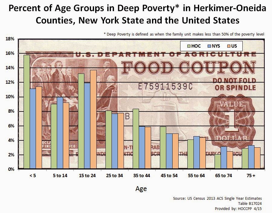
Deep Poverty Within Age Groups for the Region, NYS and the US (2013)

A continuing look at those in deep poverty. The chart below shows the percent of people in deep poverty (defined as those living in families where the income level is less than 50% of what defines poverty for that particular family structure) within various age groupings. Data from the Herkimer Oneida County region, as well as New York State and the United States, is provided.

Click to enlarge the graph for better viewing.

CLICK TO ENLARGE

Comparison of Children in Poverty 1990 Versus 2013

Recently I posted about regional children living in poverty. In that post I introduced the concepts of people living in "near poverty, "in poverty" and in "deep poverty".

"Near poverty" identifies, in this case, children under the age of 18 who live in a family where the poverty level is between 150% and 101% of poverty. So technically they are not in poverty at this time, but considered to be on the edge of poverty, or "near" poverty.

"In poverty" is for children where their family level of income is between the actual the poverty level (100% of the poverty income level) and 51% of the poverty income level.

Children in "deep poverty" are those where families are at 50% or less of the poverty levels. For these families, they are a long ways from getting out of poverty, hence the idea that they are seen as being in "deep" poverty.

The previous post just took a look at the current percentage of children in the two county area that live at each of these poverty levels. In order to provide a bit more context, here is some data that covers the regional MSA (Herkimer and Oneida Counties combined), New York State, and the United States for the years 1990 and 2013 for children in poverty. Each has seen an increase in levels of poverty pretty much across the board.

Please NOTE: In order to get the percentage of children living in poverty as more traditionally defined, you would simply add the percentages of the bottom two segments on the graph below - that is, add the percent of those in "deep poverty" to the percent "in poverty". 

Regional Children in Poverty: Kids In "Near Poverty", "In Poverty" and In "Deep Poverty"

We often talk about people, and especially children, in poverty. Not all levels of poverty are seen the same. Most government measures of poverty identify three levels, or depths, of poverty: "near poverty", "in poverty", and "deep poverty".

"Near poverty" identifies, in this case, children under the age of 18 who live in a family where the poverty level is between 150% and 101% of poverty. So technically they are not in poverty at this time, but considered to be on the edge of poverty, or "near" poverty.

"In poverty" is for children where their family level of income is between the actual the poverty level (100% of the poverty income level) and 51% of the poverty income level.

Children in "deep poverty" are those where families are at 50% or less of the poverty levels. For these families, they are a long ways from getting out of poverty, hence the idea that they are seen as being in "deep" poverty.

The graphic below shows depth of poverty among all children age 17 and under in the region. While a total of around 27% are actually below poverty, you can see how a large portion of the 27% are in deep poverty (11%). In addition, another 16.0% are hovering near poverty.

The Relationship Between Poverty, Educational Attainment, and Gender

The two graphics below show the poverty rates for persons age 25 and over in Herkimer County. The first one is for ALL people age 25 and over based on education attainment; the second breaks the educational attainment categories into males and females. This allows the viewer to see the impact of not having an high school degree, for example, on both men and women when it comes to being in poverty.

Click to enlarge either graphic.

Click to Enlarge

Click to Enlarge

Herkimer County Poverty Measures By Municipality (2013)

The 2013 ACS Five Year Estimates also provide poverty data, which many agencies use for grant writing and program preparation. The table below contains several age based poverty measures for every level of municipality in Herkimer County, including cities, towns, villages and census designated places. In addition, each of the towns where villages are incorporated are also shown without the village populations - note the towns where the name is followed by "(minus villages)". The ability to pull the village populations out of the towns allows for a closer look at our rural areas and their needs when it comes to poverty.

The age groups include: those under age 5; those under age 18, and those age 65 or older. Click on the table to enlarge it.

Herkimer County Poverty Measures (2013)

Click to Enlarge

How The Census Bureau Measures Poverty

The US Census Bureau offers two measures of poverty. The official measure of poverty is the more traditional piece based on a 1963 definition of poverty living based largely on cash resource availability. The second measure is the Supplemental Poverty Measure (SPM) which accounts for non-cash benefits from government programs aimed at low income families as well as cash resources of the household.

Below is an infographic comparing the two measures which helps explain their differences more fully. A publication by the Census Bureau, located here, provides some comparisons between the official and SPM data by state. To see local information for your community on poverty, visit this previous post of poverty and income by municipality.


[Source: U.S. Census Bureau]

An Example of Using ACS Estimates Over Time: Poverty and Family Types 2005 to 2013

As the single year (and the three year) American Community Survey (ACS) data continues to be released, it is important to remember that data now exists going back to 2005 for our area. One of the hopes of the Census Bureau was that such data availability would allow policymakers, as well as the public, the opportunity to look at their region longitudinally, albeit with a certain amount of caution.

As an example, below are the historical estimates of poverty by family type, in this case single mom families versus two parent families in Oneida County. Not surprisingly, poverty rates for single parents are quite a bit higher than they are for dual parent families - the average over the nine years is about 30% for single moms and around 5.5% for dual parent families.

Click to Enlarge

What's important to note is the trends depicted by the shaded areas in the chart, which represent the margins of error for each year. As can been seen, they are rather large for single moms and fairly small for dual parents. This is mainly because of the small number of single mom's sampled (due to their fairly small number within the community). Just be sure to take a look at those margins of error as you explore the ACS data as there are times that they are exceedingly large, and should then be viewed with a some caution.

2010 Oneida County Retrospective: Income and Poverty (Part 2)

Income Measures: Changes in income on the family, household and per capita levels have been considerable over the last 50 years. Income, in all of its various measures, has grown dramatically, increasing by more than 8  times over what it was in 1960. Per capita income, for example, has gone from a level of about $2,000 in 1960 to more than $25,000 in 2010.

Click to Enlarge

Family Income Quintiles: Income growth over the last fifty years wasn’t necessarily uniform among all members of the county.  Looking at changes in the growth of family income by quintile can shed some light onto some of these disparities. Even for the lowest quintile, income growth has been significant since 1960. While the mid-value of the lowest family income quintile was around $2,400 in 1960, by the year 2010 it had risen to nearly $17,000. 

There has been, in fact, substantial income growth for all of the county’s families since 1960. As suggested above, Oneida County families in the lowest quintile have seen their income grow by more than 700% over the last 50 years. In comparison those families comprising the top two quintiles have had income growth of 1100% over the same period. 

Click to Enlarge

2010 Oneida County Retrospective: Income and Poverty (Part 1)

Income and Poverty in Oneida County 2010

Of the many measures of how well a community is doing economically, income and poverty are two of the most common indicators of economic health.

Income Measures: Income is generally measured in three ways within the census data: household income, family income, and per capita income. Each measures three very different things. Household data measures the cumulative income of all those people within a housing unit; family income reflects the income earned by a family unit’s members; and per capita income is the total cumulative income of a geographical area divided evenly by the total number of all the persons, regardless of age, living there.(Note: For purposes of this report, income levels for 2010 are based on the 2012 Five Year ACS data, using the 2010 year as a midpoint of this grouped data set).

As a general matter, median family income tends to be higher than median household income. In comparison, per capita income is lower than either family or household income. This is understandable given that every person is included in its calculation, including those not earning income such as children, the elderly, or the infirmed. According to the ACS 2012 Five Year Estimates, median household income was about $49,148 in Oneida County. Median family income, on the other hand, was $62,232. Per capita income was around $24,890.

Click to Enlarge

Family Income Quintiles: Income quintiles are another way to look at family income. They provide information about the lowest, as well as the highest, income brackets within Oneida County. Each grouping represents a fifth of the families in the county. Looking at the income ranges of each quintile provides insight into the income level needed for a family to move upward to a higher income group. For example, among those in the bottom quintile, a family would have to earn in excess of $28,662 to move from the “low” income class to a “lower-middle” income class. “Middle” income class families, in comparison in Oneida County, earn basically from $51,729 to as much as $84,729. Families in the middle class would need to earn close to $85,000 to move up a bracket. To be part of the upper most quintile, or “upper” income class, a family would have to earn in excess of $112,000. 

Back to the Future2: The Release of the 2010 County Retrospectives

Often times data lays dormant for years, or in some cases decades, with little or no comprehensive review being undertaken to place current information in any historical context. One of the most sought after but often underutilized resources of such time series data is the decennial census. In December of 2004, the Herkimer Oneida Counties Comprehensive Planning Program released a report on the last 50 years of census related data for both Herkimer and Oneida Counties.

The time has come for the re-release of this series, updated with data from 2010. Given changes to the decennial census, the data source for much of this comparison now comes from the American Communities Survey, or the ACS. The ACS is NOT the equivalent of the decennial census. It is a very different vehicle for data collection. However, to the degree possible, comparative data will be offered.

Such a review of data is, by the very nature of such time constrained data collection, and the introduction of a new source of data (the ACS), of fraught with pitfalls. Changing definitions, as well as the nature of the data collection process itself, often conspire to make many comparisons the equivalent of mixing apples with oranges. As the social constructs of race, poverty, aging, etc., all evolve to better, or perhaps at least different, levels of understanding over the years, the ability to make comparisons with past data becomes tricky, perhaps difficult, and even impossible at times.

These report will attempt to recognize those potential issues and bring them to light. They will involve data collected since the 1950 census through the 2012 ACS Five Year Estimates. In many cases, in terms of the historical sections of each chapter, the data may only extend back to 1960 or 1970 until the 2012 ACS. Much of that is due to the introduction of new concepts (such as poverty) or a change in the basic definitions and collection of data on an issue, such as race. Sometimes, issues are only able to be examined in a broad context, such as white versus non-white populations. But there are many topics in which the data does allow for direct comparison over several decades with little change in how the data was collected or coded.

Still, it is important to strongly urge that each of the data sets be examined in terms of the subtleties of the definitions for each topical issue. Efforts have been made to be sure to compare like items when possible, and to note potential problem areas. All of the included analysis provides at least a loose sketch of the immediate historical past, and, at best, a more thorough review of some of the changes being experienced within Oneida County over the last fifty to sixty years. 

These reports are not intended as an assessment of demographic trends in the last half of the 20^th century in either county. Rather they are more of a simple review of what has occurred. While a plethora of other topics could have been included, few have enough historical context (i.e. data available) to make them readily reviewable. As a result, this report focuses on five topics: aging, families, income/poverty, nativity/race, and employment.

Expect to see these chapters released here in the next several weeks (one will be later today!). Oneida County's chapters will be released first and then Herkimer County's will follow. 

Tracking Poverty By Age Group: 1970 to 2010

A recent article I read about poverty suggests that while the "war on poverty" has been successful, it has somewhat stagnated as well. During President Johnson's term in office, the war on poverty helped raise millions above the poverty line: the poverty rate dropped from 23 percent to 12 percent.

But where do we stand today? The government's official measure of poverty shows that poverty has actually increased slightly since the Johnson administration, rising from 14.2 percent in 1967 to 15 percent in 2012.

Interestingly, information from the Columbia Population Research Center shows how national poverty rates have changed over time since the late 1960s, and in particular how these have changed for various age groups as well. They specifically looked at poverty rates among children, working age population, and the elderly over the last 45 years or so. Below is a graph showing the poverty rates for each of those age groups since 1967.

Click to Enlarge

This chart suggests that the poverty rate for the elderly has fallen, as has child poverty rates, since 1967. But the working-age poverty rate has stayed flat for 40 years. It dropped from 20 percent in 1967 to about 15 percent in 1974, and remains there today.

Locally, the patterns are a bit different, as seen below.

Click to Enlarge

Click to Enlarge

In both counties, poverty rates among the elderly do appear to have fallen over the last 40 years, similar to national data trends. However, poverty among children, those under the age of 18, has risen and risen sharply particularly since 1990. And while national poverty rates among those of "working age" (between 18 and 64)has been relatively stagnant, regionally these rates have seen a steady climb since 1970.

2012 Income and Poverty Data for Municipalities in Herkimer and Oneida Counties

With the release of the Five Year ACS Estimates in December, it is now possible to get data for every municipality in the region, regardless of size. Below are two tables (click to enlarge them) which have income and poverty data for each municipality in Herkimer and Oneida Counties. If you'd like to see other data for either county as a whole, visit the ACS matrix link.

Herkimer County Data

Click to Enlarge

Oneida County Data

Click to Enlarge

The Rise (?) of Single Parenting Nationally and Locally

Recently I came across this article from the PEW Research Center about the "Rise of Single Fathers".  As they point out in the article:

“A record 8% of households with minor children in the United States are headed by a single father, up from just over 1% in 1960, according to a Pew Research Center analysis of Decennial Census and American Community Survey data.

The number of single father households has increased about nine-fold since 1960, from less than 300,000 to more than 2.6 million in 2011.1 In comparison, the number of single mother households increased more than fourfold during that time period, up to 8.6 million in 2011, from 1.9 million in 1960.

As a result, men make up a growing share of single parent householders.2 In 1960, about 14% of single parent households were headed by fathers, today almost one-quarter (24%) are.”

When you look at the local data on family types with minor children in the home, you find some interesting trends as well. Just like the national data, we have seen a rise in the percent of families with minor children being headed by single parents. Between 1970 and 2010, the percent of families with children under the age of 18 who were headed by a single mom or dad went from about 11% to 35% in Oneida County, and in Herkimer County it rose from 9% to about 34%. These are three to four fold increases in the percentage of families experiencing single parenting.

Click to Enlarge Herkimer County Data

Click to Enlarge Oneida County Data

Obviously these increases correspond to decreases in the percentage of families with children under the age of 18 present that are headed by two parents. While in 1970 around 90% of the families with minor children were two parent families, by 2010 this number had dropped to below 65% in both counties.

I also looked at the median family incomes of these various "families with minor children present" configurations by examining the three year estimates from the American Communities Survey data for 2011. Not surprisingly married couple families with minor children at home make considerably more than their single parent compatriots.

In Herkimer County the median family income for a two parent family with minor children present is slightly above $65,000 a year; in Oneida County it was over $77,000 annually. In comparison, female headed families with minor children present only had median incomes of about $28,000 in Herkimer County and $23,000 in Oneida County.

Click to Enlarge

 Interestingly, families with minor children that were headed by single males had median incomes that were more than 40% higher than those headed by single females. Single fathers with minor children at home had median incomes of roughly $39,000 in Herkimer County – 42% higher than their female counterparts. In Oneida County, single dad families had a median income of around $33,000, or 45% higher than female headed families with minor children at home. Having only a single adult wage earner clearly makes it more difficult for single parent families to make ends meet regardless of the gender of the parent.

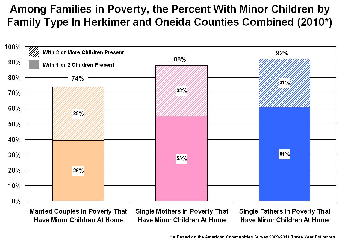
This was clearly indicated when I looked at poverty data for each type of "family with minor children at home" in our region. Examining the combined data of Herkimer and Oneida Counties, and focusing on families in poverty, we find that for all three family types (married couples, single female and single male headed families) the data shows the presence of minor children in the home is exceeding common among those in poverty. In other words it is very common in our region for families struggling with poverty to have young children at home.

Among married couples in poverty, for example, 74% of all such families have 1 or more minor children at home.  As many as a third of married couples in poverty (35%) have 3 or more children living in the household.

Click to Enlarge

In comparison, we find a larger percentage of single parent families in poverty having minor children living in the household. About 88% of all single-mom families in poverty have children under the age of 18 living at home, and 92% of all single-dad families in poverty also have minor children in the household. In both these cases about a third (33% and 31%, respectively) have three or more children present.

So while our area has seen some similarity in the "rise" of single parenting, and specifically in terms of single father families, these families are still clearly struggling when ti comes to making ends meet.